Email Spam Classification using Naive Bayes.

In this article, we will be using a dataset that contains the subject of the mail and also specifies whether the mail is spam or not based on 1 and 0 mentioned.

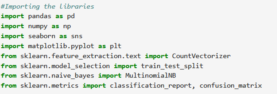
Step 1: Importing Libraries

Each of the library imported is used for the following tasks:

Pandas: Data manipulation and analysis library for working with labeled and relational data.
NumPy: Fundamental package for numerical computing with support for multidimensional arrays and mathematical functions.
Seaborn: Statistical data visualization library providing a high-level interface for creating attractive graphics.
Matplotlib: Comprehensive plotting library for creating static, interactive, and animated visualizations in Python.
scikit-learn: Machine learning library providing tools for classification, regression, clustering, dimensionality reduction, and model evaluation

step 2: Import the Dataset

It reads the data from a CSV file named ’emails.csv’ into a Pandas DataFrame named spam_df.
pd.read_csv(): This function is provided by Pandas to read data from CSV files and create a DataFrame.

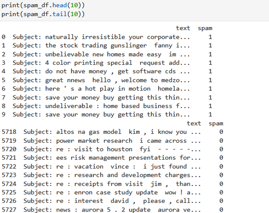
To see the first and last rows of the dataset use the head and the tail method.

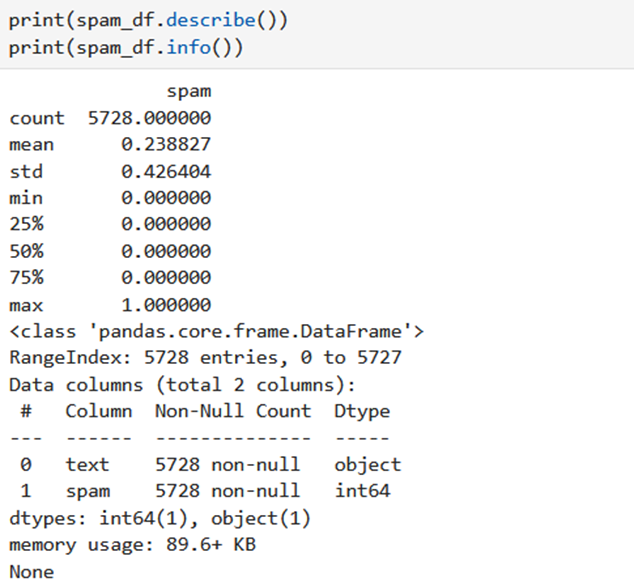
To get detailed information about the dataset you can use the describe and info method.

spam_df.describe(): generate descriptive statistics of the numerical columns in your DataFrame spam_df. It includes count, mean, standard deviation, minimum, maximum, and various percentiles of numeric data.
spam_df.info() display a concise summary of the DataFrame spam_df, including the number of non-null values and data types for each column. It helps understand the structure of your dataset, including the presence of missing values and the data types of each feature.

Step 3: Calculate the percentage of spam and ham (non-spam) emails in your dataset:

We have created a DataFrame ham containing only the rows where the ‘spam’ column equals 0, indicating non-spam emails.
Then created a DataFrame spam containing only the rows where the ‘spam’ column equals 1, indicating spam emails.
Then we calculated the percentage of spam and non-spam.

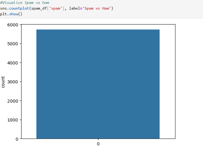
To visualize the plot you can use the seaborn library

This chart is looking at your email data and separating the emails into two categories: spam and ham.

On the left side (usually labeled 0), you have the “ham” emails. These are the normal emails you want in your inbox.
On the right side (usually labeled 1), you have the “spam” emails. These are the unwanted advertising or junk emails.

The height of each bar shows how many emails there are in each category. In your data, it seems there are more “ham” emails (taller bar) than “spam” emails (shorter bar). This helps visualize the balance between desired and unwanted emails in your dataset.

Step 4: Text Vectorization with Count vectorizer

vectorizer = CountVectorizer(): This line creates an instance of the CountVectorizer class from scikit-learn. This class is used to convert text data into numerical features.
.fit_transform(spam_df[‘text’]): This line applies the fit_transform method to the vectorizer object. It does two things:

Fit: The vectorizer analyzes the text data in the ‘text’ column of spam_df to identify unique words (vocabulary). This process is called fitting.
Transform: The vectorizer then converts each email in the ‘text’ column into a numerical feature vector. This vector represents the frequency (count) of each word in the vocabulary appearing in that email. The output is stored in a new sparse matrix called spamham_countVectorizer.

.get_feature_names_out(): This line calls the get_feature_names_out method on the vectorizer object. This method returns the vocabulary (unique words) identified during the fitting process. These vocabulary words become the feature names in the transformed sparse matrix.

It will reveal the number of emails (rows) and the number of unique words (features or columns) in your dataset after vectorization with CountVectorizer.

5728 (rows): This indicates the number of emails in your original dataset. There are likely 5728 emails that were vectorized using CountVectorizer.
37303 (columns): This represents the number of unique words (features) identified by CountVectorizer in the email text data. After transforming the text data, the resulting matrix has 37303 columns, each corresponding to a unique word found in the emails.

Step 5: Training the model

X = spamham_countVectorizer: This line assigns the previously created sparse matrix spamham_countVectorizer (containing the numerical features) to the variable X. This matrix will be used as the feature set for the model.
y = spam_df[‘spam’]: This line extracts the ‘spam’ column from the spam_df DataFrame and assigns it to the variable y. This column contains the labels (0 for ham and 1 for spam) which will be used as the target variable for the model.
.shape: This method is called on both X and y to print their shapes. The shape of a matrix indicates the number of rows and columns.

Step 6: Splitting the dataset into Training and Testing datasets

It splits the data you prepared earlier (features X and labels y) into training and testing sets.

X_train: This variable will store the training features (a subset of the original X).
X_test: This variable will store the testing features (another subset of the original X).
y_train: This variable will store the training labels (a subset of the original y corresponding to the training features in X_train).
y_test: This variable will store the testing labels (a subset of the original y corresponding to the testing features in X_test).

test_size=0.2: This argument specifies the proportion of data to be used for the testing set. In this case, 0.2 represents 20%, so 80% of the data will be allocated to the training set and 20% to the testing set.

random_state=42: This argument sets a seed for the random number generator used to split the data. This ensures reproducibility – if you run the code again with the same random_state, you’ll get the same split.

Step 7: Training a Naive Bayes classifier for spam email classification.

NB_classifier = MultinomialNB(): This line creates an instance of the MultinomialNB class from scikit-learn. This class implements the Multinomial Naive Bayes algorithm, a popular choice for text classification tasks.
.fit(X_train, y_train): This line trains the Naive Bayes classifier using the training data (X_train features and y_train labels). During training, the classifier learns the statistical relationship between the features (words) in emails and their corresponding spam/ham labels.

Step 8: Evaluating the model

y_predict_train = NB_classifier.predict(X_train): This line uses the trained Naive Bayes classifier (NB_classifier) to predict spam/ham labels for the emails in the training data (X_train). The predictions are stored in the y_predict_train variable.

Evaluating the Model on Training Data (using Confusion Matrix):

cm_train = confusion_matrix(y_train, y_predict_train): This line calculates the confusion matrix for the model’s performance on the training data. The confusion matrix compares the actual labels (y_train) with the predicted labels (y_predict_train). It shows how many emails were correctly classified as spam (true positives – TP), ham (true negatives – TN), incorrectly classified as spam (false positives – FP), and incorrectly classified as ham (false negatives – FN).

For evaluating the performance on the Testing data.

Step 9: Classification Report

Leave a Reply Cancel reply