We will be using the Social network ad dataset The dataset contains the details of users in a social networking site to find whether a user buys a product by clicking the ad on the site based on their salary, age, and gender.

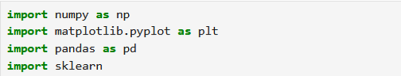
Step 1: Import Libraries

Let’s start by importing essential libraries:

Step 2: Importing a Dataset

Importing of the dataset and slicing it into independent and dependent variables:

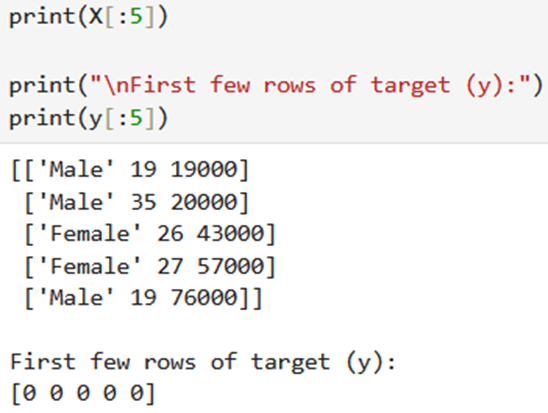
• X: This extracts the features from columns with indices 1, 2, and 3:
  • Column 1: Gender (e.g., ‘Male’, ‘Female’)
  • Column 2: Age (e.g., 19, 35, 26, …)
  • Column 3: EstimatedSalary (e.g., 19000, 20000, 43000, …)
• y: This extracts the target variable from the last column (Purchased), which indicates whether the user bought the product (1) or not (0)

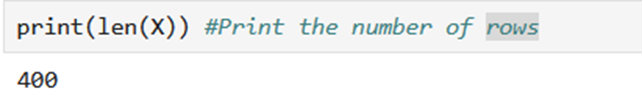
To print the length of the feature matrix ( X ), you should call the `len()` function

To print the first few rows of the dataset, you have to use the head() method.

Printing the first few rows of the features(X) and the target variable(y)

Step 3: Encode LabelEncode

Since our dataset contains character variables we have to encode it using LabelEncoder:

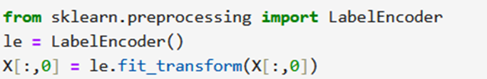
• LabelEncoder is used to convert categorical data into numerical labels.
• Then we initializes a LabelEncoder object named le.
• X[:, 0] selects all rows of the first column of the feature matrix X, which likely represents categorical data (e.g., ‘Male’, ‘Female’).
• le.fit_transform() fits the encoder to the data in the selected column and transforms the data into numerical labels.
• The transformed numerical labels are then assigned back to the corresponding column in the feature matrix X.

Step 4: Train Test and Split on Dataset

We are performing a train test split on the dataset. We are providing the test size as 0.20, that means our training sample contains 320 training set and test sample contains 80 test set.

1. X: The feature matrix containing the independent variables.
2. y: The target variable containing the dependent variable.
3. test_size = 0.20: This parameter specifies the proportion of the dataset to include in the test split. Here, 20% of the dataset will be used for testing.
4. random_state = 0: This parameter sets the random seed for reproducibility. It ensures that the data is split in the same way every time the code is run, which is important for reproducible research.

Outputs:

1. X_train: This variable contains the features for the training set.
2. X_test: This variable contains the features for the testing set.
3. y_train: This variable contains the target values for the training set.
4. y_test: This variable contains the target values for the testing set.

Next, we are doing feature scaling to the training and test set of independent variables for reducing the size to smaller values:

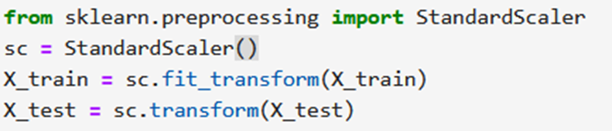
StandardScaler is a tool from the scikit-learn library used to standardize or normalize data. It adjusts the data so that it has a mean of 0 and a standard deviation of 1.

Standardizing data can help many machine learning algorithms perform better because it ensures that all features are on a similar scale. This is important for algorithms that rely on distances or gradients, such as k-Nearest Neighbors (k-NN) and Gradient Descent-based algorithms.

1. The StandardScaler is a tool used for scaling features, which means transforming data so that it fits within a specific scale.
2. we create an instance of the StandardScaler class and store it in the variable sc. This object will be used to scale our data.
3. sc.fit_transform(X_train):
4. sc.fit() computes the mean and standard deviation for each feature in the training set X_train.
5. sc.transform() then applies these computed mean and standard deviation to transform (scale) the training set X_train. This ensures that all features have a mean of 0 and a standard deviation of 1.
6. Then we only apply the transformation (scaling) to the test set X_test. We use sc.transform() instead of sc.fit_transform() because we want to use the mean and standard deviation computed from the training set to scale the test set. This ensures consistency in scaling between the training and test sets.

Step 5: Training KNN Model

Now we have to create and train the K Nearest Neighbor model with the training set:

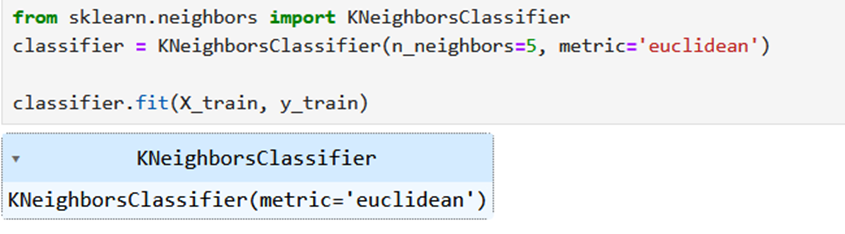
Imported the KNeighborsClassifier is a type of supervised learning algorithm used for classification tasks.

• Then we created an instance of the KNeighborsClassifier class and assigns it to the variable classifier.
• n_neighbors=5: This parameter specifies the number of neighbors to consider when making predictions. Here, we’re using 5 neighbors.
• metric=’euclidian’: This parameter specifies the distance metric used to measure the distance between points. In this case, we’re using the euclidian distance metric.
• Then we trains (fits) the KNN classifier using the training set (X_train, y_train).
• The fit() method takes the training data as input and learns from it to make predictions.

To predicts the target variable for the test set using the trained K Nearest Neighbors (KNN) classifier

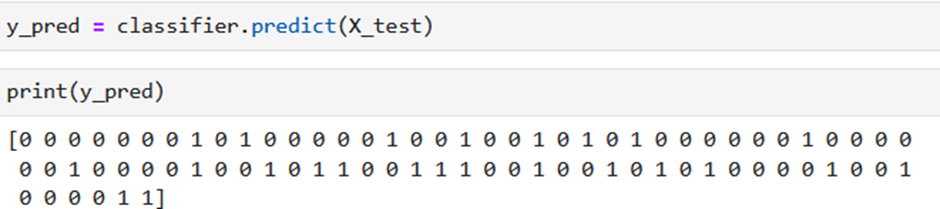
• classifier: This is the trained K Nearest Neighbors (KNN) classifier that was previously created and trained on the training data.
• .predict(): This method is used to make predictions on new data. It takes the test features (X_test) as input and returns the predicted target variable.
• X_test: This is the test set containing the independent variables (features) for which predictions are to be made.
• print(y_pred) will output the predicted target variable values stored in the y_pred variable. Each value in y_pred corresponds to the predicted target variable value for a corresponding row in the test set X_test. For example, if y_pred contains [0, 1, 1, 0, 1, …], it means that the model predicted the first test sample to belong to class 0, the second test sample to belong to class 1, the third test sample to belong to class 1, and so on.

Step 6: Evaluating the model

We can evaluate our model using the confusion matrix and accuracy score by comparing the predicted and actual test values:

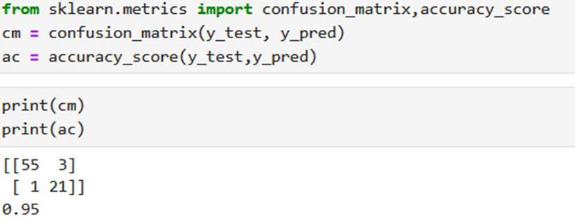
• confusion_matrix(y_test, y_pred): This function computes the confusion matrix to evaluate the accuracy of a classification. It takes the true target values (y_test) and the predicted target values (y_pred) as input and returns a confusion matrix.
• accuracy_score(y_test, y_pred): This function calculates the accuracy of the classification model by comparing the true target values (y_test) with the predicted target values (y_pred). It returns the accuracy score, which is the fraction of correctly predicted samples.

The confusion matrix has four values:

• 55: True negatives (TN) – the number of correctly predicted negative instances (actual negative instances correctly predicted as negative).
• 3: False positives (FP) – the number of incorrectly predicted positive instances (actual negative instances incorrectly predicted as positive).
• 1: False negatives (FN) – the number of incorrectly predicted negative instances (actual positive instances incorrectly predicted as negative).
• 21: True positives (TP) – the number of correctly predicted positive instances (actual positive instances correctly predicted as positive).
• The accuracy score is 0.95, indicating that the model correctly predicted 95% of the samples in the test set.

Similar Topics

Text Preprocessing: Lemmatization and Stop-words

Stemming Techniques using NLTK Library

Exploring Different Tokenization Techniques in NLP using NLTK Library